Week 9

Improving the results

Introduction

This post will cover the improvements done to the image in order to get better matches between them. It will also cover some code improvement.

Normalisation

Following Cristian’s findings, the images were normalised using CLHE (Contrast Limited Histogram Equalization). This is just a version of CLARHE (Contrast Limited Adaptive Histogram Equalization) that uses the whole images instead of patches [1]. It is already implemented in OpenCV. This has removed the shining lights from the images.

Code

def normaliseImg(img):
    height, width = np.shape(img)[:2]
    clahe = cv2.createCLAHE(clipLimit = 4, tileGridSize = (height, width))

    yuv = cv2.cvtColor(img, cv2.COLOR_BGR2YUV)
    luminance = yuv[:, :, 0]
    yuv[:, :, 0] = clahe.apply(luminance)

    return cv2.cvtColor(yuv, cv2.COLOR_YUV2BGR)

Results

Norm PCB1	Norm PCB2

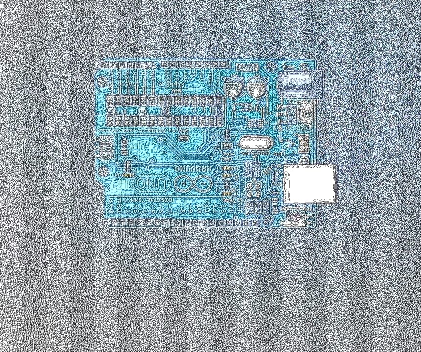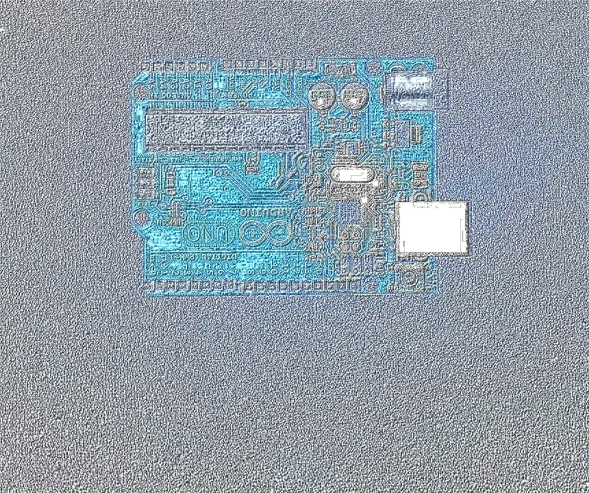Lowest Template Matching Value

In last week’s blog template matching was used to eliminate false differences found using feature matching. The normalised values of the template matching algorithms return a value between 0 (different image) to 1 (same image). This new function loops through some of the possible values from 0 to 1 to find the lowest threshold where differences were found. This way the threshold does not have be manually set.

Code

def getBestPatchesAuto(sourceImg, checkImg, patches):
    for th in range(10):
        threshold = th / 10.0
        bestPatches = getBestPatches(normPCB1, normPCB2, patches, threshold)
        if len(bestPatches) > 0:
            return bestPatches
    return bestPatches

Morphological Transformations

The mask of the differences was changed slightly to provide a more universal method of combining the different pixels.

shape = cv2.getStructuringElement(cv2.MORPH_RECT, (3, 3))
mask = cv2.dilate(mask, shape, iterations = 10)
shape = cv2.getStructuringElement(cv2.MORPH_RECT, (3, 3))
mask = cv2.erode(mask, shape, iterations = 20)

Rotating Images

As the template matching algorithm is sensitive to rotation and scaling, the two images need to have the same orientation. As the rotation angle can be found from the feature detection algorithm the only step necessary is to rotate them. More information can be found on Emmet’s blog posts [2], [3].

Results from the improvements

While the surrounding rectangle is still not perfect, it contains a smaller rectangle than before.

Differences

Conclusion

This week’s blog concentrated on improving the algorithm so it can be used for other images as well. It has also slightly improved on the test images.

References

[1] N.M. Sasi, V.K. Jayasree, Contrast Limited Adaptive Histogram Equalization for Qualitative Enhancement of Myocardial Perfusion Images, 2013, Scientific Research Publishing, p. 327

[2] E.Doyle, Rotating the Image, 2017, [Online]. Available: https://vzat.github.io/comparing_images/emmet/rotating_the_image.html. [Accessed: 2017-11-11].

[2] E.Doyle, Adding and Removing Borders, 2017, [Online]. Available: https://vzat.github.io/comparing_images/emmet/adding_and_removing_borders.html. [Accessed: 2017-11-11].